Transform Your Data: Expert Tips on Using the Pandas Melt Function Effectively

In the realm of data manipulation and analysis, reshaping data is a fundamental task. The Pandas library in Python, a powerhouse for data manipulation, offers various functions for reshaping data, one of which is the melt function. This function is incredibly useful for transforming data from a wide format to a long format, a process often referred to as unpivoting.

Understanding the Melt Function

The melt function in Pandas is primarily used for unpivoting a DataFrame. Unpivoting transforms the data from a wide format, where information spreads across many columns, to a long format, where it’s presented in a more normalized structure with rows. This transformation is particularly useful in scenarios where you need to perform operations that are more suited to a long-format structure, such as certain types of data visualization or statistical modeling.

1. Basic Usage of Melt

Let’s consider a basic example to understand how melt works. First, we’ll create a simple DataFrame. Suppose we have data representing sales figures for two products (Product A and Product B) across three months (January, February, March). The DataFrame will be in a wide format, which we will then transform to a long format using the melt function. Here’s the script:

import pandas as pd



# Create a DataFrame

data = {

    'Month': ['January', 'February', 'March'],

    'Product A': [100, 150, 200],

    'Product B': [90, 120, 160]

}



df = pd.DataFrame(data)

print("Original DataFrame:")

print(df)



# Using melt to transform the DataFrame

melted_df = df.melt(id_vars=['Month'], var_name='Product', value_name='Sales')



print("\nMelted DataFrame:")

print(melted_df)

Output:

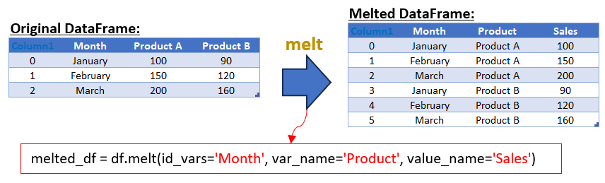
In the melted DataFrame, we have three columns: ‘Month’, ‘Product’, and ‘Sales’. The id_vars parameter in the melt function is used to specify the column(s) that you want to keep unchanged (in this case, ‘Month’). The var_name parameter is used to name the new column that will contain what were previously column headers (‘Product A’ and ‘Product B’), and value_name is used to name the new column that will contain the corresponding values (‘Sales’).

Variations in Using Melt

The flexibility of the melt function allows for several variations and additional parameters to fine-tune the data reshaping process:

• Multiple ID Variables: You can specify multiple columns in id_vars if you want to keep more than one column fixed while melting the rest of the DataFrame.
• Customizing Column Names: By adjusting var_name and value_name, you can customize the column names in the resulting long-format DataFrame to suit your data context better.
• Selective Melting: You can also specify a subset of columns to be melted using the value_vars parameter. This is particularly useful when dealing with wide-format data where only a few columns need to be transformed.
• Combining with Other Pandas Functions: Melt can be combined with other Pandas functions like sort_values, query, or groupby for more advanced data manipulation.

2. Melting Multiple ID Variables

Typically, in a melting operation, the id_vars parameter is used to specify the column(s) that you want to remain unchanged. These columns act as identifiers for the rest of the data during the transformation process. However, the real power of melt lies in its ability to accept multiple columns in id_vars. This feature allows you to keep more than one column fixed while melting the rest of the DataFrame.

Practical Applications

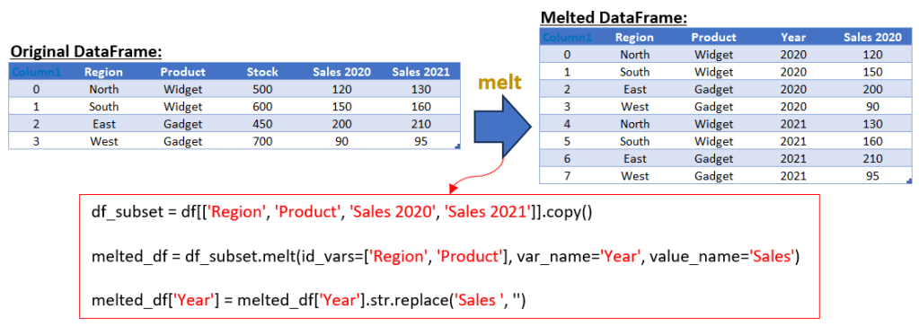
Imagine a dataset that encapsulates sales figures for various products across different regions, detailed annually. In its original wide format, this dataset presents each combination of product and region with distinct columns for each year’s sales. Such a format, while comprehensive, can be cumbersome for certain types of analysis. By applying the melt function to this dataset, with ‘Region’ and ‘Product’ as multiple ID variables, we can efficiently transform it into a long format. This reshaped dataset now aligns each region and product with corresponding sales data for each year in separate rows. This streamlined transformation not only simplifies the dataset but also optimizes it for more effective analysis, particularly beneficial for time series assessments and comparative studies across various product types and regions. The exclusion of the ‘Stock’ column in this process further refines the data, focusing the analysis strictly on sales trends over time. Here’s an example:

import pandas as pd



# Sample data: Sales figures and stock for two products across different regions over two years

data = {

    'Region': ['North', 'South', 'East', 'West'],

    'Product': ['Widget', 'Widget', 'Gadget', 'Gadget'],

    'Stock': [500, 600, 450, 700],

    'Sales 2020': [120, 150, 200, 90],

    'Sales 2021': [130, 160, 210, 95]

}



# Creating a DataFrame from the data

df = pd.DataFrame(data)

print("Original DataFrame:")

print(df)



# Creating a subset of the DataFrame without the 'Stock' column

df_subset = df[['Region', 'Product', 'Sales 2020', 'Sales 2021']]



# Using melt to transform the subset DataFrame

# 'id_vars' specifies the columns to keep fixed (Region and Product in this case)

melted_df = df_subset.melt(id_vars=['Region', 'Product'], var_name='Year', value_name='Sales')



# Cleaning up the 'Year' column to remove the 'Sales ' prefix

melted_df['Year'] = melted_df['Year'].str.replace('Sales ', '')



print("\nMelted DataFrame:")

print(melted_df)

Output:

Explanation of the Script:

1. Data Preparation: The script starts with the same DataFrame df that includes sales data and stock levels.
2. Creating a Subset DataFrame: Before melting, a new DataFrame df_subset is created, which includes all columns from df except for the “Stock” column. This is done by selecting only the ‘Region’, ‘Product’, ‘Sales 2020’, and ‘Sales 2021’ columns.
3. Melting the Subset DataFrame: The melt function is then applied to df_subset. Since df_subset does not include the “Stock” column, it will not appear in the melted DataFrame. The id_vars are set to ‘Region’ and ‘Product’, and the sales data columns are unpivoted into ‘Year’ and ‘Sales’.
4. Output: The final melted DataFrame, melted_df, is printed, showing the long format data with ‘Region’, ‘Product’, ‘Year’, and ‘Sales’, excluding the stock information.

By creating a subset DataFrame that excludes the “Stock” column, this script ensures that the stock data does not appear in the final melted DataFrame, focusing solely on the sales data across regions and products.

3. Melting Multiple Value Columns

Let’s consider an example where you have a DataFrame with multiple value columns and you want to melt it. Suppose you have a DataFrame with sales and profit data for two products across three months:

import pandas as pd



# Define sample data: Sales and Profit for Product A and B across three months

data = {

    'Month': ['January', 'February', 'March'],

    'Sales Product A': [100, 150, 200],

    'Profit Product A': [20, 30, 40],

    'Sales Product B': [90, 120, 160],

    'Profit Product B': [10, 15, 25]

}



# Create a DataFrame from the provided data

df = pd.DataFrame(data)

print("Original DataFrame:")

print(df)



# Melt the DataFrame for Sales data

# 'id_vars' keeps the 'Month' column unchanged

# 'value_vars' specifies which columns to melt (here, Sales data columns)

# 'var_name' is the name of the new column for melted 'variable' names (Product names)

# 'value_name' is the name of the new column for values corresponding to the melted 'variable' names (Sales figures)

sales_melted = df.melt(id_vars=['Month'], value_vars=['Sales Product A', 'Sales Product B'], 

                       var_name='Product', value_name='Sales')

# Clean up the 'Product' column by removing the 'Sales ' prefix, leaving only the product names

sales_melted['Product'] = sales_melted['Product'].str.replace('Sales ', '')



# Repeat the melting process for Profit data

profit_melted = df.melt(id_vars=['Month'], value_vars=['Profit Product A', 'Profit Product B'], 

                        var_name='Product', value_name='Profit')

# Similarly, clean up the 'Product' column by removing the 'Profit ' prefix

profit_melted['Product'] = profit_melted['Product'].str.replace('Profit ', '')



# Merge the melted Sales and Profit DataFrames

# The merge is based on the 'Month' and 'Product' columns, which are common to both DataFrames

combined_melted = pd.merge(sales_melted, profit_melted, on=['Month', 'Product'])



# Display the final combined DataFrame

print("Melted DataFrame:")

print(combined_melted)

Output:

Explanation of the Script:

1. Data Preparation: The script starts by importing the pandas library. Then, it defines a dictionary data containing sales and profit figures for two products (Product A and Product B) across three months (January, February, March).
2. Creating the Original DataFrame: This dictionary is converted into a pandas DataFrame named df, which is then printed to the console. This DataFrame is in a wide format, where each row represents a month, and separate columns are dedicated to sales and profit figures for each product.
3. Melting the DataFrame for Sales: The DataFrame is melted using the melt function to transform the sales data from a wide format to a long format. The id_vars parameter is used to keep the ‘Month’ column fixed, while the value_vars parameter specifies the columns that contain the sales data. The var_name and value_name parameters are used to name the new columns created by the melt operation. The ‘Product’ column is then cleaned to remove the ‘Sales ‘ prefix, leaving only the product names.
4. Melting the DataFrame for Profit: A similar melting process is applied to the profit data. The DataFrame is melted to transform the profit data, and the ‘Product’ column is cleaned to remove the ‘Profit ‘ prefix.
5. Combining Melted DataFrames: The two melted DataFrames (sales_melted and profit_melted) are then merged into a single DataFrame combined_melted based on the ‘Month’ and ‘Product’ columns. This merged DataFrame represents a long format where each row contains the month, product name, sales figure, and profit figure.
6. Output: Finally, the script prints the combined melted DataFrame, showcasing the data in a format that is often more suitable for analysis and visualization tasks.

4. Selective Melting

A particularly useful aspect of melt function is its ability to perform selective melting, which is achieved through the value_vars parameter. This feature allows for the transformation of only a specified subset of columns, enhancing efficiency and focus on data reshaping tasks. Selective melting is a process where only certain columns of a DataFrame are unpivoted, while others are either retained as identifier variables or excluded from the transformation. This is particularly advantageous when dealing with wide-format data that contains numerous columns, out of which only a few are relevant for a specific analysis.

The Role of value_vars in Selective Melting

The value_vars parameter in the melt function allows you to specify which columns should be melted. By default, if value_vars is not specified, all columns not set as id_vars are melted. However, by explicitly defining value_vars, you can limit the melting process to only those columns that are essential for your analysis, thereby streamlining the data transformation process.

Practical Example

Consider a dataset that includes sales, stock, and customer feedback scores for various products over multiple years. Suppose you are only interested in analyzing the sales and stock data, and want to exclude the feedback scores from the melting process.

Here’s how you can apply selective melting to this dataset:

import pandas as pd



# Sample data: Sales, Stock, and Feedback Scores for products over two years

data = {

    'Product': ['Widget', 'Gadget'],

    'Sales 2020': [120, 200],

    'Sales 2021': [130, 210],

    'Stock 2020': [500, 450],

    'Stock 2021': [600, 700],

    'Feedback Score 2020': [4.5, 4.7],

    'Feedback Score 2021': [4.6, 4.8]

}



# Creating a DataFrame from the data

df = pd.DataFrame(data)

print("Original DataFrame:")

print(df)



# Using melt to selectively transform Sales and Stock data

melted_df = df.melt(id_vars=['Product'], value_vars=['Sales 2020', 'Sales 2021', 'Stock 2020', 'Stock 2021'], 

                    var_name='Metric', value_name='Value')



print("\nSelectively Melted DataFrame:")

print(melted_df)

Output:

Output Explanation:

• Data Preparation: The script starts with a DataFrame df that includes sales, stock, and feedback score data.
• Applying Selective Melting: The melt function is used with id_vars set to ‘Product’ and value_vars specified to include only the sales and stock columns for both years. The feedback score columns are thus excluded from the melting process.
• Result: The final DataFrame melted_df displays the long-format data with ‘Product’, ‘Metric’, and ‘Value’, focusing solely on the sales and stock information.

Selective melting, as demonstrated, allows for targeted data transformation, making it an invaluable technique for handling wide-format datasets with precision and relevance to specific analytical needs.

5. Integrating Melt with Pandas’ Data Manipulation Toolkit

While melt is a powerful tool for reshaping data, its true potential is unleashed when combined with other Pandas functions. This integration enables analysts to perform complex data transformations and analyses more efficiently.

1. Melt and Sort_Values: By combining melt with sort_values, you can reshape your data and then immediately sort it based on certain criteria, such as sorting sales data by date or value after melting.
2. Melt and Query: The query function can be used post-melting to filter the dataset based on a condition, providing a streamlined way to narrow down your data for specific analyses.
3. Melt and GroupBy: Perhaps one of the most powerful combinations is using melt with groupby. This allows for the aggregation of melted data based on certain categories, which is particularly useful in statistical analysis and reporting.

Practical Example

Let’s consider a dataset containing sales and stock figures for various products. We’ll first melt the data and then demonstrate how it can be sorted, queried, and grouped for different analytical purposes.

import pandas as pd



# Sample data: Sales and stock figures for products

data = {

    'Product': ['Widget', 'Gadget', 'Thingamajig'],

    'Sales 2020': [120, 200, 150],

    'Sales 2021': [130, 210, 160],

    'Stock 2020': [50, 60, 40],

    'Stock 2021': [55, 65, 45]

}



# Creating a DataFrame from the data

df = pd.DataFrame(data)

print("Original DataFrame (df): ")

print(df)



# Melting the DataFrame

melted_df = df.melt(id_vars=['Product'], var_name='Year and Metric', value_name='Value')

print("Melted DataFrame:")

print(melted_df)



# Sorting the melted DataFrame by Value

sorted_df = melted_df.sort_values(by='Value', ascending=False)



# Filtering the melted DataFrame for Sales data of 2021

sales_2021_df = melted_df.query("`Year and Metric` == 'Sales 2021'")



# Grouping the melted DataFrame by Product and aggregating values

grouped_df = melted_df.groupby('Product').sum()



print("Sorted Melted DataFrame:")

print(sorted_df)

print("\nFiltered Melted DataFrame for Sales 2021:")

print(sales_2021_df)

print("\nGrouped Melted DataFrame by Product:")

print(grouped_df)

Output:

Output Explanation:

• Sorting: The sort_values function is used to sort the melted DataFrame by the ‘Value’ column, allowing for a quick overview of the highest figures across all metrics and years.
• Filtering: The query function filters the data to show only the sales figures for the year 2021, providing a focused view of that particular year.
• Grouping: The groupby function aggregates the data by ‘Product’, summing up all sales and stock figures, which is useful for understanding the total figures per product.

By integrating melt with other Pandas functions, we can perform a range of data manipulation tasks more efficiently, making it an invaluable approach for complex data analysis scenarios.

Conclusion

Throughout this exploration of the Pandas melt function, we’ve delved into various facets of this versatile tool, uncovering its potential to transform and enhance data analysis. From the basic usage of melt for simple data reshaping to its integration with other powerful Pandas functions, we’ve seen how melt can be a pivotal part of a data analyst’s toolkit.

The journey began with understanding the fundamental operation of melt in converting data from a wide format to a long format, a crucial step in preparing data for in-depth analysis. We then explored advanced applications, including the use of multiple ID variables to maintain the integrity of complex datasets during transformation, and the customization of column names to improve data readability and context.

Selective melting emerged as a particularly effective strategy for focusing on specific data segments, enhancing efficiency and analytical precision. This approach is invaluable when dealing with extensive datasets where only certain columns are pertinent to the analysis.

Moreover, the integration of melt with other Pandas functions like sort_values, query, and groupby opened new avenues for data manipulation. This synergy allows for a seamless workflow, from reshaping and sorting data to filtering and aggregating it, thereby enabling more comprehensive and insightful analyses. In conclusion, Pandas’ melt function is not just a tool for reshaping data; it’s a gateway to a broader realm of data manipulation possibilities. By mastering melt and its complementary functions, analysts and data scientists can unlock new levels of efficiency and insight in their data exploration journey. Whether it’s for preparing datasets for visualization, statistical modeling, or machine learning, the effective use of melt can significantly streamline the data preprocessing workflow, paving the way for more informed decision-making and impactful data storytelling.