Pandas, a powerful data manipulation library in Python, offers various functions for reshaping and analyzing data. One such function is pivot_table, which is incredibly useful for summarizing and analyzing complex datasets. However, the default column names generated by pivot_table might not always be intuitive or suitable for your analysis. In this guide, we’ll explore how to customize column names in Pandas pivot tables for clearer and more meaningful data representation.
1. Basic Pivot Table with Custom Column Names
Imagine you’re analyzing sales and profit data for an electronics store. You have data categorized by date and product category, and you’re interested in summarizing the total and average sales and profits for each category on each date. Here’s how you start by creating a DataFrame:
import pandas as pd


# Sample data representing sales and profit for different categories over two dates

data = {

    'Date': ['2021-01-01', '2021-01-01', '2021-01-01', '2021-01-02', '2021-01-02', '2021-01-02'],

    'Category': ['Electronics', 'Electronics', 'Clothing', 'Electronics', 'Electronics', 'Clothing'],

    'Sales': [200, 210, 150, 230, 220, 180],

    'Profit': [20, 25, 15, 23, 22, 18]

}


# Creating a DataFrame from the sample data

df = pd.DataFrame(data)

print("Original DataFrame (df):")

print(df, end="\n\n")
Next, you create a pivot table to aggregate this data. The pivot_table method is used to calculate the sum and mean for both sales and profit. However, the default column names like ‘Sales_sum’ and ‘Sales_mean’ may not be immediately intuitive. Customizing these names can make your data more understandable:
# Creating a pivot table with multi-level aggregation

pivot_table_multi = df.pivot_table(index=['Date', 'Category'], values=['Sales', 'Profit'], aggfunc={'Sales': ['sum', 'mean'], 'Profit': ['sum', 'mean']})


# Customizing the column names for clarity

pivot_table_multi.columns = ['_'.join(col).strip() for col in pivot_table_multi.columns.values]

pivot_table_multi = pivot_table_multi.rename(columns={

    'Sales_sum': 'Total Sales',

    'Sales_mean': 'Average Sales',

    'Profit_sum': 'Total Profit',

    'Profit_mean': 'Average Profit'

})


print("DataFrame After Customizing Column Names:")

print(pivot_table_multi)
Now, let’s integrate the above script to appear as follows:
import pandas as pd


# Sample data representing sales and profit for different categories over two dates

data = {

    'Date': ['2021-01-01', '2021-01-01', '2021-01-01', '2021-01-02', '2021-01-02', '2021-01-02'],

    'Category': ['Electronics', 'Electronics', 'Clothing', 'Electronics', 'Electronics', 'Clothing'],

    'Sales': [200, 210, 150, 230, 220, 180],

    'Profit': [20, 25, 15, 23, 22, 18]

}


# Creating a DataFrame from the sample data

df = pd.DataFrame(data)

print("Original DataFrame (df):")

print(df, end="\n\n")


# Creating a pivot table to aggregate sales and profit data by date and category

# The pivot_table method is used with sum and mean as aggregation functions

pivot_table_multi = df.pivot_table(index=['Date', 'Category'], values=['Sales', 'Profit'], aggfunc={'Sales': ['sum', 'mean'], 'Profit': ['sum', 'mean']})


# Displaying the pivot table after aggregation

print("DataFrame After Pivoted:")

print(pivot_table_multi, end="\n\n")


# Customizing the column names for better clarity and understanding

# The column names are concatenated and then renamed to more descriptive titles

pivot_table_multi.columns = ['_'.join(col).strip() for col in pivot_table_multi.columns.values]

pivot_table_multi = pivot_table_multi.rename(columns={

    'Sales_sum': 'Total Sales',

    'Sales_mean': 'Average Sales',

    'Profit_sum': 'Total Profit',

    'Profit_mean': 'Average Profit'

})


# Displaying the DataFrame with customized column names

print("DataFrame After Customizing Column Names:")

print(pivot_table_multi)
Output:

This script demonstrates the process of creating a pivot table in Pandas for aggregating data, followed by customizing the column names to enhance readability and clarity. Initially, the pivot_table method is employed to calculate both the sum and mean of ‘Sales’ and ‘Profit’ for each ‘Category’ across different ‘Dates’. The resulting pivot table has multi-level column headers, which are tuples combining the aggregation function (like ‘sum’ or ‘mean’) with the data column (‘Sales’ or ‘Profit’). These multi-level headers are then transformed into single-level headers by concatenating the tuple elements using an underscore. This is achieved using the list comprehension [‘_’.join(col).strip() for col in pivot_table_multi.columns.values], which joins the elements of each tuple in the multi-level header and creates a flat list of column names. Finally, the rename method is used to replace these concatenated names with more descriptive titles, such as changing ‘Sales_sum’ to ‘Total Sales’ and ‘Sales_mean’ to ‘Average Sales’. This customization of column names makes the aggregated data in the pivot table more understandable and meaningful for analysis.
2. Advanced Pivot Tables: Customizing Multi-Level Column Names
In this section, we’ll explore an advanced pivot table scenario where we deal with multiple columns in the ‘columns’ parameter. This approach is particularly useful when analyzing data across various dimensions, such as region and type, in addition to the primary categories and dates. Let’s dive into the script:
import pandas as pd


# Sample data with an additional 'Type' column

data = {

    'Date': ['2021-01-01', '2021-01-01', '2021-01-01', '2021-01-02', '2021-01-02', '2021-01-02'],

    'Category': ['Electronics', 'Electronics', 'Clothing', 'Electronics', 'Electronics', 'Clothing'],

    'Region': ['North', 'South', 'North', 'South', 'North', 'South'],

    'Type': ['Type1', 'Type2', 'Type1', 'Type2', 'Type1', 'Type2'],

    'Sales': [200, 210, 150, 230, 220, 180],

    'Profit': [20, 25, 15, 23, 22, 18]

}


# Creating a DataFrame from the sample data

df = pd.DataFrame(data)

print("Original DataFrame (df):")

print(df, end="\n\n")


# Creating a pivot table with multi-level aggregation across multiple dimensions

pivot_table_multi = df.pivot_table(index=['Date', 'Category'], columns=['Region', 'Type'], values=['Sales', 'Profit'], aggfunc={'Sales': ['sum', 'mean'], 'Profit': ['sum', 'mean']})


# Displaying the pivot table after aggregation

print("DataFrame After Pivoted:")

print(pivot_table_multi, end="\n\n")


# Customizing the column names for better clarity and understanding

pivot_table_multi.columns = ['_'.join(col).strip() for col in pivot_table_multi.columns.values]


# Displaying the DataFrame with customized column names

print("DataFrame After Customizing Column Names:")

print(pivot_table_multi)
Output:
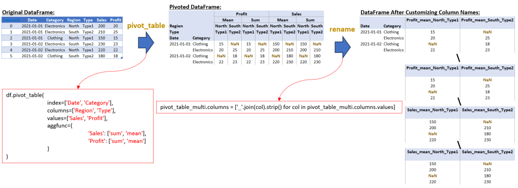
In this script, we first create a DataFrame with additional dimensions ‘Region’ and ‘Type’. We then use the pivot_table method to perform a multi-level aggregation. This method allows us to set multiple columns as indices (‘Date’ and ‘Category’) and define multiple columns in the columns parameter (‘Region’ and ‘Type’). This creates a comprehensive table that can be used for in-depth analysis across different segments and time periods.
In this section, we deal with a more complex pivot table that involves multiple columns in the ‘columns’ parameter, resulting in a multi-level column structure. After creating the pivot table, the multi-level column names are concatenated to form single-level column names. This is done by joining the elements of each tuple in the multi-level header with an underscore, using a list comprehension like [‘_’.join(col).strip() for col in pivot_table_multi.columns.values].
This process transforms the multi-level column names into a single, flattened structure. For example, a multi-level column header like (‘Sales’, ‘sum’, ‘North’, ‘Type1’) and (‘Sales’, ‘mean’, ‘North’, ‘Type1’) would be concatenated to ‘Sales_sum_North_Type1’ and ‘Sales_mean_North_Type1’.
The key point here is that we are not only customizing the column names for clarity but also handling a more complex structure due to the multi-level nature of the columns in the pivot table. This process is crucial for making the data more interpretable and insightful, especially when working with advanced data structures.
Conclusion
In this guide, we’ve explored the powerful capabilities of Pandas’ pivot_table function, focusing on how to enhance data clarity through customizing column names. This skill is essential for data analysts and scientists who often work with complex datasets and need to present their findings in an understandable and insightful manner.
In Section 1, “Basic Pivot Table with Custom Column Names,” we demonstrated how to transform a simple pivot table’s default column names into more descriptive titles. This step is crucial for making aggregated data like total and average sales and profits more interpretable. By renaming columns like ‘Sales_sum’ to ‘Total Sales’ and ‘Sales_mean’ to ‘Average Sales’, we significantly improved the readability of our pivot table, making it easier for anyone to understand the data at a glance.
Moving to Section 2, “Advanced Pivot Tables: Customizing Multi-Level Column Names,” we tackled a more complex scenario involving multiple dimensions like region and type. Here, the pivot_table‘s multi-level column structure presented a unique challenge. We addressed this by first flattening the multi-level column names into a single level, allowing for a more streamlined and readable format. This step is crucial for making the data more interpretable, especially when working with complex, multi-dimensional datasets. The renaming of these columns for enhanced clarity can be done based on your specific analytical requirements, by following the approach demonstrated in Section 1.
Through these examples, it’s evident that customizing column names in pivot tables is not just a matter of aesthetics but a critical step in data analysis. It ensures that the insights derived from the data are accessible and actionable. As we continue to delve into the world of data manipulation with Pandas.
